Modeling Number of Coronavirus Cases with Logistic Growth
If you have been following the news recently, you may have heard of the spread of the Novel coronavirus 2019-nCoV. The growth in the number of cases poses some open questions: how many cases will we expect in the future, and at what point can we expect the number of new infections to plateau? In this post, I’ll attempt to answer these questions with mathematical modeling. With only a basic understanding of calculus and some calculations easily done in a spreadsheet, we can perform very accurate modeling of a very complicated natural phenomenon!
In school, we are typically given a function and then asked to calculate some properties about the function. For example, we might be asked to compute the value of the function for some given input:
However, in the real world, we do not always have access to the underlying function.
Instead, we might be given some observations about the world, and we want to use this data
to try to find an approximation to the original function that might have generated
those observations. For example,
we have the data about (date, total number of coronavirus cases) for the past
several weeks, and we want to find the function that best matches the data.
Once we have this equation, we can use it to predict the projected number of cases in the future. This process is very common in machine learning settings, where the process of estimating the parameters for the function is called training, and using the function to predict new values is called inference.
For example, in a machine learning setting, the function we try to estimate might be a probability distribution: given an email, what is the probability that it is spam? Training samples allow us to estimate the probability distribution model, and this probability distribution allows us to perform inference on future emails to determine if they are spam.
The challenge with mathematical modeling is figuring out the right model to use that captures the underlying phenomenon we are observing, and then estimating the parameters for those models. In this post, I’ll talk about why a logistic growth model [1] can be used to model the number of coronavirus cases, and how we can estimate the parameters of the logistic growth model to infer number of cases in the future.
Primer about differential equations
We can use a differential equation to understand the intuition behind the logistic growth model. For readers unfamiliar with differential equations, this section provide some intuition behind them.
As a functional programmer [2] at heart, the best way I understand new concepts is to first understand the types involved. In the normal equations one typically sees in school, the solution to the equations are usually a set of values in the real numbers or complex numbers. For example, the solution to the following equation:
is the set of real numbers
For a differential equation, the solution to the equation is a set of functions. For example, for the following differential equation where $r$ is a constant and $P$ is a function of $t$:
this equation means that both sides are equal for all values of $t$. The solution to this differential equation is a family of functions:
for all constants $P_0$. We can take the derivative to double check that it satisfies the differential equation:
Logistic growth differential equation
The differential equation above models exponential growth. As an example, we can imagine $P(0)$ as the population of bunnies at time $t = 0$. Given infinite resources in the environment, suppose each bunny has $r = 2$ bunnies as offspring every year. Then in the next year, we expect there to be $rP(0) = 2 * P(0)$ additional bunnies, for a total of $P(1) = rP(0) + P(0)$ bunnies at time $t = 1$. In the second year, we expect there $rP(1) = 2 * P(1)$ additional bunnies, for a total of $P(2) = rP(1) + P(1)$ total bunnies, and so on.
More generally, given a population size $P$ at time $t$, and a growth rate $r$, we expect the net change in total number of bunnies over some period of time, represented as the derivative, to be the following:
However, the real world is constrained: there is not be enough food in the environment to support unlimited growth in bunnies. As more bunnies enter the population and the environment gets saturated, the growth in the number of additional bunnies added year over year should start to decrease. To constrain the growth, we add an additional constraining factor into the differential equation:
where $K$ is the maximum size the population will ever be. This differential equation models logistic growth.
When $P$ is small, the right factor will be close to 1, and this function will approximate exponential growth. When $P$ grows and starts to approach $K$, the right factor will start to approach 0, and this causes the rate of growth to decrease. The solution to this differential equation is the family of functions
for all constants $P_0$. Here, $P_0$ represents the starting population size at time $t = 0$.
Similar to population growth in a constrained environment, the logistic growth equation can also be used to model number of infected people with the novel coronavirus. During the initial outbreak, the number of cases grow exponentially. As more people became infected and people enter quarantine, the infection starts to saturate, as there are fewer new people to be infected.
For more intuition and interesting properties about the logistic growth model, I highly recommend watching this youtube video from the Veritasium channel [3] – this channel is great for learning interesting scientific and mathematical phenomenon, and is what inspired me to write this post!
The rest of this post will discuss how we model the number of coronavirus cases over time using a logistic growth model. Our goal is the following:
1) Using the current data available about (date, total number of coronavirus cases), we want to infer
the logistic growth parameters $r, K, P_0$.
2) Using the estimated parameters, predict the total number of coronavirus cases in the future.
Estimating Logistic Growth Parameters
Estimating $r$ and $K$
To calculate parameters $r, K, P_0$, let’s first rewrite the logistic growth differential equation by dividing both sides by $P$:
We can use the data (date, total number of coronavirus cases) to calculate the left hand side of the equation.
For example, suppose our data looked like the following:
(t, P(t))
(day 1, 100 cases)
(day 2, 200 cases)
(day 3, 400 cases)
Then we can estimate the derivative $dP/dt$ on day 2 using the following:
Dividing by $P(t)$ gives us the following:
Note that in the rewritten equation, the left hand side is proportional to the right hand side, which reminds us of linear relationships $y = mx + b$:
where $m = -r/K$ is the slope of $x = P$ with respect to $y = (dP/dt)/P$, and $b = r$ is the $y$-intercept.
To calculate the slope and the intercept, we can create a scatterplot of the calculated
$(x, y) = (P, (dP/dt)/P)$ values in our dataset, and then use a
linear regression [4] to calculate
the line of best fit for the slope and intercept. In Google Sheets, you can calculate this using
the SLOPE and INTERCEPT macros. For more information about this technique to find $r$ and $K$,
take a look at this MAA article [5].
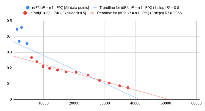
For our estimation, we used the number of coronavirus cases from January 23 to February 9, and we obtained this data from this source [6]. The figure above shows the scatterplot and the blue line represents the results of the linear regression using all the data points. Note that the first few data points are outliers compared to the rest of the data. If we ignore these data points, we can estimate a more accurate line of best fit. The Random Sample and Consensus (RANSAC) Algorithm [7] can find this automatically, however in our case, it was simple enough to eyeball it from the scatterplot and manually exclude the initial data points, and this results in the line of best fit in red.
From this linear regression, we calculated the following results for $r$ and $K$ to be the following:
This means that in our estimated model, the total number of people that will ever be infected with coronavirus will be $K = 51109$, and during the early exponential growth phase of the outbreak, each persion roughly infects $0.27$ new people per day.
Estimating $P_0$
Now that we have our estimates for $r$ and $K$, the final step is to estimate the initial starting population size $P_0$. To get some intuition on the potential values for $P_0$, I created two plots of the logistic growth function $P$ using our calculated values for $r$ and $K$, and the two plots used different initial starting population size $P_0 = 1317$ and $P_0 = 2015$. These numbers were the number of total cases as of January 24 and January 25, respectively. The figure below shows the result.
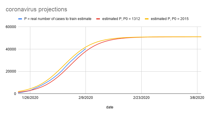
The real number of cases (shown in blue) is sandwiched between the two estimated plots, and this shows that the true value of $P_0$ is somewhere between these two values. To calculate the optimal value of $P_0$ that gives us the best-fit logistic growth, we can define an optimization problem, where the solution to the optimization problem gives us the best fit value for $P_0$.
Let $P_{est}(P_0, t)$ be the estimated total number of coronavirus cases at time $t$, using the $r$ and $K$ values we calculated earlier, and the provided input $P_0$. This estimation will probably not match exactly the real observed number of cases $P_{real}(t)$. Let
represent the error between our estimation and true number of cases at time $t$ and a given $P_0$. Here, we chose the square of the difference so that the error function is always non-negative and is differentiable (unlike the absolute value function). Next, we define the total error function:
be the sum of all the errors for all observed data points at times $t$. By making the error function always be non-negative, this allows us to reframe the search for the best $P_0$ for our logistic growth model as an optimization problem: the value of $P_0$ that minimizes the total error will be the best $P_0$ for our model.
Analytically, we can calculate the extrema (minimum and maximum) of a function by taking the derivative with respect to $P_0$ and setting it equal to 0:
However, the calculations involved in doing this derivative for all data points would be too complex. Instead, I used this python script to calculate the $\text{TotalError}(P_0)$ function for all values between our initial estimates of $P_0 = 1317$ and $P_0 = 2015$, and plotted the data in the figure below.
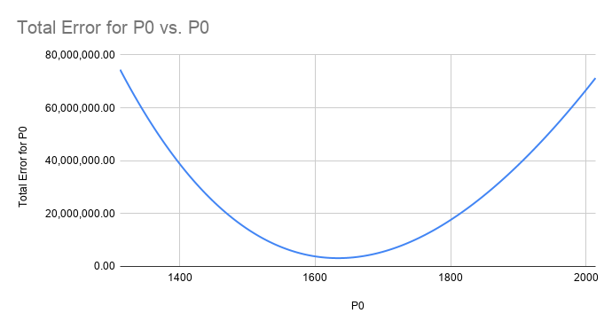
From this plot, we see that we achieve the minimum total error when
Predicting number of future Coronavirus cases
Finally, we have all the estimates for the parameters for our logistic growth model $P$.
For the data (date, total number of coronavirus cases) from January 23 to February 9,
we have the following values for our parameters:
where:
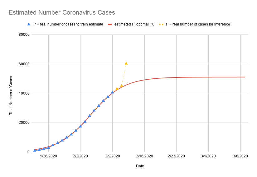
For reference, the calculations and figures were done in this Google Sheet [8]. Using these parameters in our function $P$, we can use it to predict the number of cases at a future time $t$. The figure below plots our model $P$ with the real number of cases.
Our logistic growth model $P$ is in red, the real observed data points used to estimate the model are in blue, and the new data points that have been collected since I created the model are in yellow.
For the new data points on February 10 and February 11, the prediction from our model is $1.7\%$ and $2.2\%$ off from the real reported total number of cases up to that day. Pretty good!
This model also predicts that the total number of cases will stop growing at $K = 51109$, and the daily number of new cases will be less than 100 starting on February 23.
Limitations
You probably noticed on the last figure: what happened on February 12? Why is our estimation so off on that day? Despite the initial accuracy of the logistic growth model, the model has limitations, and the real world is much more complex.
As an example, as I was writing this post, the Chinese government changed the definition of how it counts coronavirus cases, resulting in the 15,000 additional cases on February 12 in the figure above. Furthermore, the model will not take into account new outbreaks that might happen in different cities, which may result in a sudden growth in new infections. As the Lunar New Year holiday in China ends and more people start to travel again, this may also increase the rate of infection, reducing the constraining factor essential to the logistic growth model. In addition, the logistic growth model assumes a constant growth factor $r$, however, the coronavirus may behave differently in different people, and it may evolve to become more or less infectious over time.
Despite these limitations, the logistic growth model provides us with a surprisingly accurate way to model the number of coronavirus cases so far using only basic calculations that can be done in a spreadsheet!
Thanks for reading! I hope you learned something new!
Links
- [1] Logistic Growth Model
- [2] Functional Programming – A key factor in functional programming is understanding the types. The best way for me to understand new concepts is to understand the types and their relationships with each other.
- [3] Youtube video from Veritasium explaining the logistic growth equation and other interesting facts about it
- [4] Linear Regression
- [5] Logistic Growth Model: Fitting a Logistic Model to Data
- [6] Worldometer: Coronavirus Cases – This is where I obtained the
(date, number of coronavirus cases)data. In this post, I used the data from January 23 to February 9 to estimate the parameters for the model. - [7] Random Sample Consensus (RANSAC)
- [8] Google Sheet where these calulations were done